Simulate the standardised sum of independent and

Question

1. Repeatedly (10⁴ times) simulate the standardised sum of independent and identically distributed variates X₁, . . . ,X_n

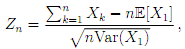
and provide histogram plots, with the (suitably renormalised) standard normal density curve superimposed, for

(a) X₁ ~ Exp(1) and n = 2, 6, 1000.
(b) X₁ ~ Ber(3=4) and n = 5, 20, 100.

Supply your code.

2. Repeat the simulation in Q1a with n = 1000, and independently simulate an equal number of outcomes from the standard normal distribution using the Box- Muller method. Plot the empirical quantiles against eachother, together with the line y = x, and comment on the plausibility that the samples come from the same distribution. Supply your code.

3. Simulate 10⁶ outcomes (X, Y ), where

with Θ ~ [0, 2Π), and R = 5 + S with S ~ Exp(1) independently of Θ. Provide a scatter plot of typical output, and give the (empirical) correlation. Comment on the correlation and dependence of (X, Y ). Supply your code.

4. Simulate 200 coin-flip experiments with success parameter p = 1=4, and compute the average number of successes p, together with an approximate 95% conβdence interval

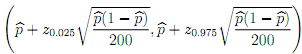
where z_q is the q-th quantile of a standard normal variate. Repeat the experiment 10⁴ times, and plot the approximate conβdence intervals for each experiment, together with a line showing the true success parameter. Calculate the proportion of the 10⁴ repeated experiments that contain the true success parameter, and comment. Supply your code.

5. Simulate N = 10³ outcomes from the model

Y = -2 + X + ε

where X ~ U[0, 1] and ε ~ N(0, 0.12 ) independently. From your simulated outcomes of (X, Y ), βt a linear regression model to increasing numbers of outcomes (from N = 2 to N = 10⁴ ) as

y = β₀ + β₁x

by using the solution to the normal equations to obtain estimates for , via solving where

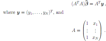
Plot your estimates for β₀ and β₁ as N increases, together with a line indicating their true values. Supply your code.

6. Simulate N = 10⁴ outcomes from the model

where X ~ U[0, 1] and ε ~ N(0, 0.1 ) independently. From your simulated outcomes of (X, Y ).

(a) Fit a linear regression model as in Q5, and plot your estimates for β₀ and β₁ as N increases, together with a line indicating their true values. Supply your code.

(b) Fit a quadratic regression model y = β₀ + β_1x+ β₂x², and plot your estimates for β₀, β₁, and β₂ as N increases, together with a line indicating their true values. Supply your code.