Discuss the below:
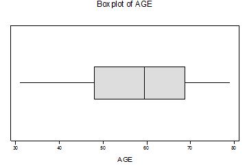
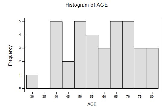
1) The age of the 36 millionaires sampled are arranged in increasing order in the tables below.
Use the Descriptive statistics output and the graphs to response the following questions:
a) Describe the distribution: Hint: Shape, Center, Spread and the outliers. be sure to interpret your answers.
b)Does your histogram support your boxplot? Explain.
c) State the five number summary and interpret.
Millionaires
|
31
|
48
|
60
|
69
|
|
38
|
48
|
61
|
71
|
|
39
|
52
|
64
|
71
|
|
39
|
52
|
64
|
74
|
|
42
|
53
|
66
|
75
|
|
42
|
54
|
66
|
77
|
|
45
|
55
|
67
|
79
|
|
47
|
57
|
68
|
79
|
|
48
|
59
|
68
|
79
|
Descriptive Statistics
Variable N Mean Median StDev SE Mean
AGE 36 58.53 59.50 13.36 2.23
Variable Minimum Maximum Q1 Q3
AGE 31.00 79.00 48.00 68.75
2) An important application of regression analysis in accounting is in the estimation of cost. By collecting data on volume and cost and using the least square method to develop an estimated regression equation relating volume and cost, an accountant can estimate the cost associated with a particular manufacturing volumes and total cost data for a manufacturing operation.
|
Production X
|
Total Cost
|
|
400
|
4000
|
|
450
|
5000
|
|
550
|
5400
|
|
600
|
5900
|
|
700
|
6400
|
|
750
|
7000
|
|
450
|
4600
|
|
420
|
4600
|
|
370
|
3900
|
|
650
|
6300
|
|
650
|
6500
|
|
610
|
6200
|
|
720
|
7300
|
|
550
|
5000
|
|
600
|
6500
|
|
800
|
8000
|
|
850
|
8200
|
|
800
|
8500
|
Use the available output and graphs below to answer the following questions:
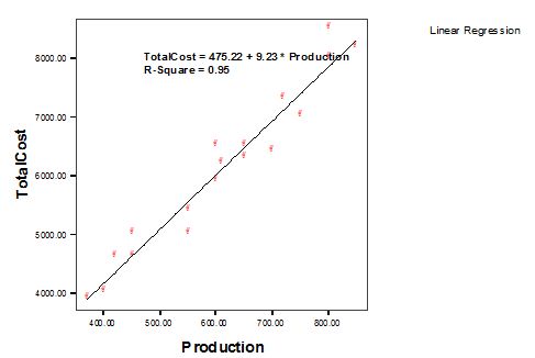
a) Explain the form, the direction and the strength of the relation ship between production and Cost.
b) State the estimated regression equation
c) Provide an interpretation for the slope of the estimated regression equation.
d) If the company's total cost next month is projected to be $7720, what will the production volume be?
e) What is the coefficient of determination r2? What percentage of the variation in total cost can be explained by production volume?
f) What is correlation coefficient r, does this number support your guess in (a)? Explain.
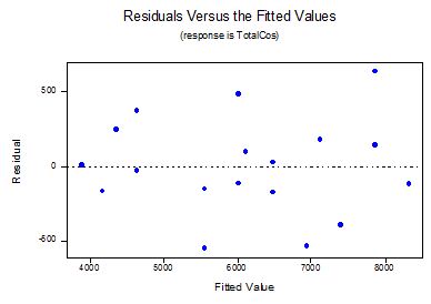
g) Did the estimated regression equation provide a good fit? Explain. Hint: r2
h) Does the residual plot support your answer in (g)? Explain.
The regression equation is
Predictor Coef StDev T P
Constant 475.2 341.1 1.39 0.183
Producti 9.2258 0.5473 16.86 0.000
S = 332.4 R-Sq = 94.7% R-Sq(adj) = 94.3%
3) Sampling distributions:
An automatic grinding machine in an auto parts plant prepares axles with a target diameter μ=40.135millimeters (mm). The machine has some variability, so the standard deviation of the diameter is σ= 0.003 mm. A sample of 4 axles is inspected each hour for process control purposes, and records are kept of the sample mean diameter. If the process mean is exactly equal to the target value, what will be the mean and standard deviation of the numbers recorded?
4) Confidence Interval:
You want to rent an unfurnished one-bedroom apartment in Boston next year. The mean monthly rent for a random sample of 10 apartments advertised in the local newspaper is $1400. Assume that the standard deviation is 220. Find a 95% confidence interval for the mean monthly rent for unfurnished one-bedroom apartments available for rent in this community. Interpret.
5) Cell phone bill
The following are the last year's local monthly bills, in dollars, for a random sample of 60 cell phone users. At 5% significance level, do the data provide sufficient evidence to conclude that last year's mean local monthly bill for cell phone users has decreased from the 1996 mean of $5025? Assume that σ = $25.
State your hypothesis, significant level α = 0.05, draw conclusion comparing p-value to α = 0.05
Use the output below to answer the questions. Don't forget to interpret and give recommendation(s)
Cell Phone Monthly Bills
|
25.07
|
42.13
|
16.74
|
16.50
|
24.86
|
35.38
|
|
77.54
|
15.83
|
29.13
|
45.00
|
23.78
|
32.09
|
|
33.21
|
32.81
|
42.37
|
35.97
|
31.93
|
40.66
|
|
31.42
|
13.85
|
17.26
|
20.28
|
48.65
|
12.90
|
|
16.46
|
15.70
|
61.64
|
29.28
|
65.01
|
12.65
|
|
104.53
|
30.42
|
45.15
|
46.87
|
50.81
|
18.18
|
|
47.98
|
14.95
|
15.45
|
28.41
|
46.57
|
46.37
|
|
62.30
|
51.95
|
58.00
|
16.89
|
81.49
|
29.00
|
|
44.07
|
127.17
|
13.81
|
49.68
|
28.37
|
43.23
|
|
117.29
|
27.43
|
22.76
|
89.28
|
35.93
|
100.80
|
Z-Test
Test of mu = 50.25 vs mu not = 50.25
The assumed sigma = 25.0
Variable N Mean StDev SE Mean Z P
BILL 60 40.69 26.25 3.23 -2.96 0.0031