Solve the following problem:
Produce several parallel MCMC chains {βtm }t,m for the pump data model as in Example 1 and study the variability of the number of simulations N proposed by raftery.diag. Compare this with the other stopping rules contained in coda.
Example 1:
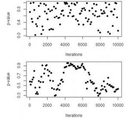
Considering again the nuclear pump failures of, we monitor the subchain (β(t) ) produced by the algorithm. Figure (top) gives the value of the Kolmogorov-Smirnov p-values produced by ks.test as T increases to 10 3. This is a sequential graph in that each dot is based on the sample of β(t)'s produced at time T and then thinned by a lag of G = 10 and separated into both halves.
Note that the Gibbs sampler is initialized at the MLE of the λi's. Since Figure (top) exhibits a lack of pattern and a fair spread of the p-value over [0, 1], there is no indication of a lack of stationarity to deduce from this graph. If instead we compare two different chains with the same tool, Figure (bottom) indicates a longer time pattern. Indeed, while the Kolmogorov- Smirnov p-values remain far away from low probabilities, the pattern exhibited in this comparison means that, while around iterations 4000 to 6000 both samples provide very similar empirical cdfs, they explore differently the space in the later iterations. Thus 10 4 iterations are not sufficient to provide a stable evaluation of the stationary distribution (for at least one chain).