Why or why not do you see any potential drawbacks to

Question

First let's investigate the quality of the asymptotic approximation discussed in the notes using a relatively small sample.

a. Write a MATLAB function called compute_standard_variance_ratio that takes two inputs, a vector of observations Y and a scalar K, and outputs the value of the estimated K-period variance ratio using non-overlapping observations. Use this function to simulate the finite-sample distribution of the K-period variance ratio for the RW1 model discussed in class. Each simulation trial should generate T+1 log prices from the model

P_t = P_t-1 + e_t

with p_O = 0 and e_t distributed 1.i.d. N(0,1), and compute the K-period variance ratio for the continuously-compounded returns. Use the command mg to set the seed for the random number generator to a value of 12345 before starting the simulation trials. Conduct a total of N-5000 trials and use (I) a histogram and (ii) a qq-plot to illustrate the distributional properties of your estimates of MVR(K)-1) for K-5, T-100. How close are the mean and variance of the finite•sample distribution to the mean and variance of the asymptotic distribution? In what percentage of the simulation trials is the null hypothesis VR(k) = 1 rejected based on a t-test at the 5% significance level using the asymptotic critical value?

b. Write a MATLAB function called compute_overlapping_variance_ratio that takes two inputs, a vector of observations Y and a scalar K, and outputs the value of the estimated K-period variance ratio using overlapping observations. Use this function to simulate the finite-sample distribution of the K-period variance ratio for the RW1 model discussed in class. Each simulation trial should generate T+1 log prices from the model

P_t = P_t-1 + e_t

with p₀-0 and e_t distributed i.i.d. N(0,1), and compute the K-period variance ratio for continuously-compounded returns. Use the command mg to set the seed for the random number generator to a value of 12345 before starting the simulation trials. Conduct a total of N-5000 trials and use (i) a histogram and (II) a qq-plot to illustrate the distributional properties of your estimates of NIT(VR(K)- 1) for K•5, Tn100. How close are the mean and variance of the finite-sample distribution to the mean and variance of the asymptotic distribution? In what percentage of the simulation trials is the null hypothesis VR(k) = 1 rejected based on a t-test at the 5% significance level using the asymptotic critical value?

c. Now consider a version of the RW3 model. In particular, each simulation trial should generate T+1 log prices from the model

 

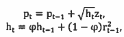
with p₀ = 0 h_o = 1, r_o = 0, and z, distributed i.l.d. N(0,1), and compute the K-period variance ratio for non-overlapping, continuously-compounded returns. Use the command mg to set the seed for the random number generator to a value of 12345 before starting the simulation trials. Conduct a total of N.5000 trials and use (I) a histogram and (II) a qq-plot to illustrate the distributional properties of your estimates of IFT(VR(K)- 1) for 9 = 0.95, K-5, T-100. Assess the impact of conditional heteroskedasticity on the test by comparing your results to those obtained In part a. In what percentage of the simulation trials is the null hypothesis VR(k) = 1 rejected based on a t-test at the 5% significance level using the asymptotic critical value?

Problem 2

Next let's examine the power of the test to detect violations of the null hypothesis under an AR(1) alternative to the random walk model.

a. Suppose the data generating process for log price differences is an AR(1) model,

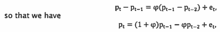
with p₀= 0, p-1 = 0, and e_t distributed N(0,1). As before, compute the K-period variance

ratio for non-overlapping, continuously-compounded returns. Use the command mg to set the seed for the random number generator to a value of 12345 before starting the simulation trials. Conduct N-5000 trials and use (I) a histogram and (ii) a qq-plot to illustrate the distribution of your estimates of .17(vR(K)- 1) for cp = 0.3, K-5, T=100. In what percentage of the simulation trials is the null VR(k) 1 rejected based on a t-test at the 5% significance level using the asymptotic critical value? Repeat the analysis for N500. How does increasing T affect the results?

b. Modify the code you wrote for part a by setting up a loop after generating the data. Use the loop to compute the fraction of rejections for each integer value of K from 2 to Kmax. Set Kmax-20 and plot the rejection fraction as a function of K with to = 0.3 and Tn100. What value of K maximizes test power? Does your answer change if you set et = -0.5 instead? Note: use the same pseudo random values of (e_t)t., to construct the returns for both values of cm This will ensure that Monte Carlo error is not driving any changes that you might see.

Problem 3.

Finally let's consider the impact of extending the random walk model by incorporating a fixed, non-zero, bid-ask spread.

a. Following Roll (1984), suppose the data generating process for log prices is

m_t= m_t-1 + e_t,

P_t = m_t + q_tc,

where the buy/sell indicator q_t which equals +1 with probability 0.5 and -1 with probability 0.5, is i.i.d. and distributed independently of m_t. Using T-1000 (instead of T=100), repeat the analysis of part a of Question 1 for data generated from this model with c=0.3, m₀=0 and e, distributed i.i.d. N(0,1). What do the results suggest about the potential importance of market microstructure effects?

b.   Under the Roll (1984) model, the bid-ask spread induces serial correlation at the first lag only. it therefore implies an MA(1) data generating process for returns. This suggests a potential way to purge the microstructure-induced autocorrelation before conducting the variance ratio test. Recall that an MA(1) model with MA parameter 0 generates a first order autocorrelation of p = 81(1 + 0²). Let fi denote the estimated first-order autocorrelation of the continuously-compounded returns. After generating the data, compute p and use the MATLAB function /zero along with the above formula to solve for 0 (the help file for (zero has examples of how to use it). Then compute the adjusted returns rt =11 - ant, for t -1,1,...,T starting with rj = 0. Next, using T=1000, repeat the analysis of part a of Question 1 for the adjusted returns Instead of the original returns. Do your results indicate that this approach works as Intended? Why or why not? Do you see any potential drawbacks to adjusting the returns to purge microstructure-induced autocorrelation?