Utility maximization consumption bundles

Question

Q1: Derive a demand curve

By knowing what bundle maximizes an individual’ s utility under various price levels, we can derive a demand curve for that person. Consider the following setup:

Situation 1: Income = $20, P_x = $5, P_y = $2

Situation 2: Income = $20, P_x = $2, P_y = $2

a) Draw the budget lines for both situations on one graph, labeling them BL₁ and BL₂.

b) Suppose we are told something about the consumer’s preferences: in situation 1 she buys X=2 and Y=5, and in situation 2 she buys X = 4 and Y = 6. Mark and label these points on the appropriate budget lines, and sketch the indifference curve that the consumer reaches in each of the two situations.

c) Set up a new graph, with “Price of X” on the vertical axis and “Quantity of X” on the horizontal axis. For each of the two prices of X that we have considered, plot the price against the quantity demanded at that price (which you can see on the previous graph). Finally, sketch a line through the points a nd label it “Demand for X.” (Assume that the demand curve for X is a straight line.)

d) For extra practice, try assuming that the price of Y changes instead of the price of X. Suppose the new situation has price levels Px = $5 and P_y = $5 (this is our “situation 3”). In this case, the individual consumes X = 1 and Y = 3. Using this information, along with the information provided for situation 1, derive the demand curve for Y. (Assume that the demand curve for Y is a straight line.)

Q2: Budget Lines and Indifference Curves

An Indifference Curve is a line that shows all the consumption bundles that yield the same amount of total utility for an individual. Please use the three types of indifference curves you learned from your lecture and the discussion section to answer the following questions.

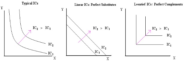
a) Suppose Jack has an income of $12 to buy two goods: sandwiches and sodas. The price of a bottle of soda is $1, and the price of a sandwich is $2. Draw Jack’s budget line (BL1) given his income is $12. (Measure sodas on the X-axis and sandwiches on the Y-axis.) Assume Jack’s utility function is U(x,y) =xy (x is the consumption amount of sodas and y is the consump tion amount of sandwiches). Jack’s marginal utility of consuming sodas and sandwiches at consumption bundle (x, y) are denoted by MUx(x, y) and MUy(x, y) respectively. Jack’s preference s are depicted by typical ICs (the left graph). The consumption bundle (x, y) which maximizes Jack’s utility satisfies:

MUx(x, y)/MUy(x, y)=y/x.

(1) Please find the numerical values of x and y of the utility maximization point (x, y). Draw a typical indifference curve (IC1) through this utility maximization point.

(2) Suppose the price of a bottle of soda increases from $1 to $4, draw Jack’s new budget lines (BL₂) and find his new utility maximization consumption bundles.

(3) Draw an imaginary budget line (BL₃) parallel to the new budget line (BL₂) and make it tangent to the initial indifference curve (IC₁). Show the income and substitution effect of the decrease in the consumption of soda as the price of soda increases. At the new price level, at least how much income should Jack get to achieve the original utility level? (Hint: find the tangent point of BL₃ and initial indifference curve (IC₁))

b) Lisa loves drinking coffee and tea. Drinking one cup of tea gives Lisa 10 utils, and drinking one cups of coffee gives he r the same utility. Suppose Lisa has an income of $12 to buy coffee and tea. The price of a cup of tea is $1, and the price of a cup of coffee is $2. Dr aw Lisa’s budget line (BL₁) given her income is $12. (Measure tea on the X-axis and coffee on th e Y-axis.) Assume that the utility from consumption of an additional unit of either good is constant (this is just a simplifying assumption to make the math easier).

(1) Please find the utility maximization point and draw an indifference curve (IC₁) through the utility maximiza tion point. (Hint: in this example, coffee and tea are perfect substitutes.)

(2) Suppose the price of a cup of tea increases from $1 to $4, draw Lisa’s new budget lines (BL₂) and find her new utility maximization consumption bundles.

(3) Draw an imaginary budget line (BL₃) parallel to the new budget line (BL₂) and make it cross the initial indifference curve (IC₁) at the lowest income level. Show the income and substitution effect of the decrease in the consumption of tea as the price of tea increases.

c) Mary is a student in the Math departme nt who has a lot of math homework. In doing the math homework she will use pencils (assume these pencils have no erasers on their ends) to make all her cal culations and an eraser to correct her answers. Mary knows that for every 2 pencils, 1 eraser will be needed. Any more pencils will serve no purpose, because she will not be able to erase the calculations. The price of an eraser is $2, and the price of a pencil is $1. Draw Mary’s budget line (BL1) given her income is $12. (Measure pencils on the X-axis and erasers on the Y-axis.)

(1) Please find the utility maximization point and draw an indifference curve (IC₁) through the utility maximization point. (Hint: in this example, pencils and erasers are perfectly complements).

(2) Suppose the price of a pencil increase s from $1 to $4, draw Mary’s new budget lines (BL 2 ) and find her new utility maximization consumption bundles.

(3) Draw an imaginary budget line (BL₃) parallel to the new budget line (BL₂) and make it cross to the initial indifference curve (IC₁) at the lowest income level. Show the income and substitution effect of the decrease in the consumption of pencils as the price of pencils increase.

Q3: Production Cost I

The following table gives cost information for a firm. Assume that labor is paid a constant wage and capital is paid a constant price, i.e., our firm is a price-taker both in the labor and capital markets.

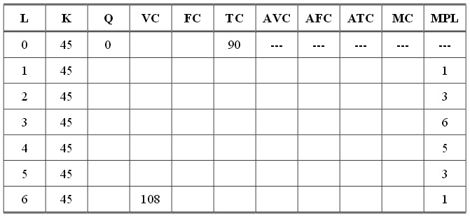
Note: L is labor; K is capital; Q is output; VC is variable cost; FC is fixed cost; TC is total cost; AVC is average variable cost; AFC is average fixed cost; ATC is average total cost; MC is marginal cost; and MPL is the marginal product of labor.

a) Please explain when output is equal to zero, why does the firm still incur costs in the short run? What is the fixed cost of this firm?

b) What is the wage rate? What is the price of a unit of capital?

c) Please complete the above table with specific numbers (compute your answer to one place past the decimal).

d) At what level of output and labor usage does marginal cost attain its minimum?

e) At what level of output and labor usage is AVC at its minimum?

f) At what level of output and labor usage is ATC at its minimum?

g) At what level of labor usage does the law of diminishing returns first occur?

h) As output increases, why does AVC first decrease, but then eventually increase? Please explain your answer.

i) Suppose the price of output is $18, fill in the following table using the information you gathered in the above table.

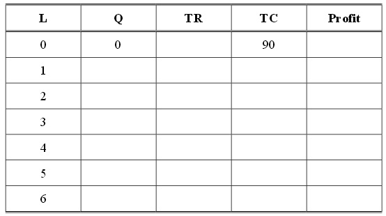
j) At what production level does the firm get its maximum profit? Please explain your answer.

Q4: Production Cost:

II The figure below shows three curves, MC, ATC and AVC, for the firm in a perfectly competitive market. In this market, the price of the good is $10. Use the information given in the figure to answer the following questions.

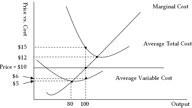
a)

(1) In the short run, will t he firm shut down the production when price equals 10?

(2) If the firm does not shut down in the short run when price equals 10, will the firm make a positive economic profit or a negative economic profit? What is the value of the firm's economic profit wh en price equals 10?

(3) If the firm does not shut down in the short run when price equals 10, what will be the firm's production level? Calculate the firm's fixed cost and variable cost at this level of production.

b) What is the break-even price for the firm? What is the shut-down price for the firm?

Q5: Perfect Competition The market for study desks is characterized by perfect competition. Firms and consumers are price takers and in the long run there is free entry and exit of firms in this industry. All firms are identical in terms of their technological capabilities. Thus the cost function as given below for a representative firm can be assumed to be the cost function faced by each firm in the industry. The total cost and marginal cost functions for the representative firm are given by the following equations:

TC = 2Q_s² + 5Q_s + 50

MC = 4Q_S + 5

Suppose that the market demand in this market is given by:

P_d = 1025 - 2Q_d

a) What is the equilibrium price in this market? (Hint: since the market supply is unknown at this point, it’s better not to think of trying to solve this problem using demand and supply equations. Instead you should think about this problem from the perspective of a representative firm.)

b) What is the long-run output of each representative firm in this industry?

c) When this industry is in long-run equilibrium, how many firms are in the industry?

Now suppose that the number of students increases such that the market demand curve for study desks shifts out and is given by,

P_d = 1525 - 2Q_d

d) In the short-run will a representative firm in this industry earn negative economic profits, positive economic profits, or zero economic profits? (Hint: do no calculation.)

e) In the long-run will a representative firm in this industry earn negative economic profits, positive economic profits, or zero economic profits? (Hint: do no calculation.)

f) What will be the new long-run equilibrium price in this industry?

g) At the new long-run equilibrium, what will be the output of each representative firm in the industry?

h) At the new long-run equilibrium, how many firms will be in the industry? Now, consider another scenario where technology advancement changes the cost functions of each representative firm. The market demand is still the original one (before the increase in the number of students). The new cost functions are:

TC = Q_s² + 5Q_s + 36
MC = 2Q_s + 5

i) What will be the new equilibrium price? Is it higher or lower than the original equilibrium price?

j) In the long-run given this technological advance, how many firms will there be in the industry?