Question 1: Suppose that there is a Beta(2,2) prior distribution on the probability θ that a coin will yield a "head" when spun in a speci?ed manner. The coin is independently spun 10 times, and "heads" appears 3 times.
a) Calculate the posterior mean.
b) Calculate the posterior variance.
c) Calculate the posterior probability that .45 ≤ θ ≤ .55.
Question 2:Consider x ˜ Normal(θ,1), θ ˜ (0, 1) and the loss L(θ, δ) = e-3θΛ2/2(θ - δ)2. Derive the estimator that minimizes the posterior expected loss.
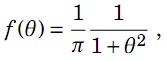
Question 3: Suppose X1, . . . ,Xn has Normal(θ,52) density and a Cauchy(0,1) prior on θ is considered. Suppose sample mean and sample variance are 25 and 49 respectively and sample size is 50. Note that the Cauchy(0,1) density is:
a) Use the Metropolis – Hastings algorithm to sample θ from the posterior distribution. Sample 10,000 θs and take the initial value θ[0] = 0. Show your R program, trace plot, acf plot, and histogram of the 10,000 θs. Give the estimate of θ2, i.e., E[θ2|X1, . . . ,Xn].
b) Use the fact,
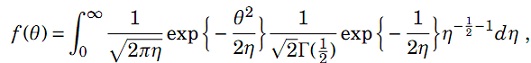
It says, conditional on η,θ has Normal(0, η) distribution and marginally, η has Inverse-Gamma(1/2,1/2) distribution. Derive the posterior distributions of θ|η,X1, . . . ,Xn and η|θ,X1, . . . ,Xn. Use Gibbs Sampler algorithms to sample θ and η iteratively from the posterior distributions. Sample 10,000 θs and 10,000 ηs and take the initial values θ[0] = 0 and η[0] = 1. Show your R program, trace plots, acf plots, and histograms of both 10,000 θs and 10,000 ηs. Give the estimate of θ2, i.e., E[θ2|X1, . . . ,Xn].
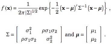
Question 4: A bivariate Normal variable x = (x1, x2)' has density
The Random Walk Metropolis – Hastings algorithm is employed to sample random variates from the distribution. A R program is listed below for the purpose.
mu1 <- 1
mu2 <- 0
sigma1 <- 1
sigma2 <- 2
rho <- 0.5
xsamples <- matrix(rep(0,2*10001),10001,2);
xsamples[1,] <- c(0,0);
for (i in 2:10001) {
Y <- xsamples[i-1,1] + rt(1,2);
U <- runif(1,0,1);
condmean <- mu1+rho*sigma1/sigma2*(xsamples[i-1,2]-mu2);
condvar <- sigma1*sigma1*(1-rho*rho);
rho0 <- min(dnorm(Y,condmean,sqrt(condvar))/
dnorm(xsamples[i-1,1],condmean,sqrt(condvar)),1);
if (U<=rho0) {
xsamples[i,1] <- Y;
} else {
xsamples[i,1] <- xsamples[i-1,1];
}
Y <- xsamples[i-1,2] + rt(1,2);
U <- runif(1,0,1);
condmean <- mu2+rho*sigma2/sigma1*(xsamples[i,1]-mu1);
condvar <- sigma2*sigma2*(1-rho*rho);
rho0 <- min(dnorm(Y,condmean,sqrt(condvar))/
dnorm(xsamples[i-1,2],condmean,sqrt(condvar)),1);
if (U<=rho0) {
xsamples[i,2] <- Y;
} else {
xsamples[i,2] <- xsamples[i-1,2];
}
}
a) Identify the parameter values for the mean and the covariance matrix of the bivariate Normal distribution according to the program.
b) State the conditional distribution of x1 given x2.
c) Briefly describe the program.