Poles on the imaginary versus real plane

Question

For this task, you will need Matlab in order to solve it ..

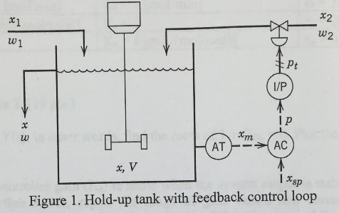
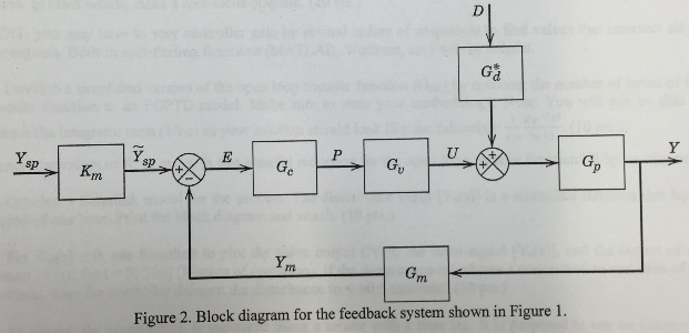
A hold-up tank is used to adjust the composition of a diluted reagent solution before it is fed into a reactor (Figure). A sample port at the bottom of the tank is used for composition measurements. Based on the measured value of composition, a PI controller will adjust the flow of pure reagent into the tank to ensure a consistent feed concentration before the contents of the tank are transferred to the reactor unit. The feedback mechanism for the tank is summarized in the illustrated block diagram (see Figure).

Assumptions:

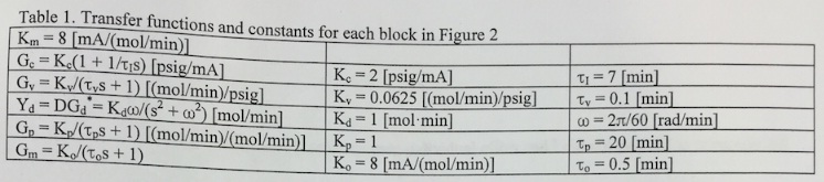
• The change in composition of the feed has been modeled and fit to a sinusoidal function (Yd
• A PI controller has been installed on the pro'cess.
• The control valve has a linear response with a nominal lag in response time (Tv)
• Diffusion and mixing has been quantitatively summarized using a first-order transfer function (GP).
• The composition of the tank is measured using a continuous inline sensor. However, there is a moderate lag in the measurement due to the dead volume of the sample port.
• Molar flow rates Ysp, Ym, Y, and Yd are measured as deviation variables from steady-state.
• Volumetric flow of make-up feed is much less than the volumetric flow of the reagent feed (q2 <

Complete the following:

1) Define Y(s) using Figure 2.

2) Determine the poles of Y(s), in other words, find the roots of 1 + G_oL, = 0. Plot the poles on the Imaginary vs. Real plane.

3) Vary the value of the controller gain (K_c) to show when the system output is stable and unstable, oscillatory and non-oscillatory. In other words, report the range of gain values that correspond to oscillatory, non-oscillatory, stable, and unstable outputs. Plot the poles for different values of K_c on the Imaginary vs. Real plane. In other words, make a root-locus diagram.

HINT: you may have to vary controller gain by several orders of magnitude to find values that intersect all of the regions. Built-in root-finding functions (MATLAB, Wolfram, etc.) will be helpful.

4) Develop a simplified version of the open loop transfer function (G_OL) by reducing the number of terms of the transfer function to an FOPTD model. Make sure to state your methodology. Note: You will not be able to reduce the integrator term (1/τ₁s) so your solution should look like the following:

(1/τ₁s) [Ke^-td^s/τs + 1]

Report the values of K, t_d, and τ. Is this a useful reduction for the open-loop transfer function? Why or why not?

5) Develop a Simulink model for the process. The disturbance input [Y_d(s)] is a sinusoidal function that has a period of one hour. Print the block diagram and attach.

6) For Y_sp(s) = 0, use Simulink to plot the valve output [P(s)], the input signal [Y_d(s)], and the output of the system [Y(s)] for t = [0 300] (5 hours of operation). If the disturbance introduces a concentration variation of ±1 mol/min, does the controller dampen the disturbance to < ±0.5 mol/min?

7) As shown, the composition is measured using a sensor with a time lag. It is proposed to use an automated sampler and gas chromatograph (GC) as a more accurate method to determine composition. Replace the current transfer function (G_m) with a time-delay transfer function (K_oe^-td^s) in the Simulink model (HINT: Use transfer delay and gain blocks). Assume K_o is the same gain for the original sensor.

What is the maximum analysis time (t_d) for the GC that can be incorporated into this feedback loop before it becomes unstable?

What are the advantages and disadvantages of using a compositional sensor like a GC? Will a GC be usable for this application? Why or why not.