Measures of variation

Question

Discuss the below:

Measures of Variation

1. Find the range, mean, variance, and standard deviation of the population data set.

a. 11 10 8 4 6 7 11 6 11 7

b.  13 23 15 13 18 13 15

14 20 20 18 17 20 1

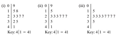
1. Without calculating, which data set has the greatest sample standard deviation? Which has the least sample standard deviation? Explain your reasoning.

2. How are the data sets the same? How do they differ?

Water Consumption The number of gallons of water consumed per day by a small village are listed. Make a frequency distribution (using five classes) for the data set. Then approximate the population mean and the population standard deviation of the data set.

167	180	192	173	145	151	174	175	178	160
195	224	244	146	162	146	177	163	149	188

Use frequency distribution formulas to approximate the sample mean and standard deviation of the following data set 

108	139	120	123	120	132	123	131	131	157	150	124	111
101	135	119	116	117	127	128	139	119	118	114	127	Â

Weekly salaries (in dollars) for a sample of registered nurses are listed.

774

446

1019

795

908

667

444

960

1. Find the mean, the median, and the mode of the salaries. Which best describes a typical salary?
2. Find the range, variance, and standard deviation of the data set. Interpret the results in the context of the real-life setting.

Confidence Intervals for the Mean (Small Samples)

Suppose you incorrectly used the normal distribution of find the maximum error of estimate for the given values of c, s, and n.

1. Find the value of E using the normal distribution.
2. Find the correct value using a t-distribution. Compare the results.

c = 0.95, s = 5, n = 16

Suppose you incorrectly used the normal distribution of find the maximum error of estimate for the given values of c, s, and n.

1. Find the value of E using the normal distribution.
2. Find the correct value using a t-distribution. Compare the results.

c = 0.99, c = 3, n = 6

1. You want to estimate the mean repair cost for dishwashers. The estimate must be within $10 of the population mean. Determine the required sample size to construct a 99% confidence interval for the population mean. Assume the population standard deviation is $22.50.

The following data set represents the repair costs (in dollars) for a random sample of 30 dishwashers.

41.82	52.81	57.80	68.16	73.48	78.88	88.13	88.79
90.07	90.35	91.68	91.72	93.01	95.21	95.34	96.50
100.05	101.32	103.59	104.19	105.62	111.32	117.14	118.42
118.77	119.01	120.70	140.52	141.84	147.06	Â	Â

Assume the population of dishwasher repair costs is normally distributed.

1. Construct a 95% confidence interval for the population variance.
2. Construct a 95% confidence interval for the population standard deviation.

An auto maker estimates that the mean gas mileage of its luxury sedan is at least 25 miles per gallon. A random sample of eight such cars had a mean of 23 miles per gallon and a standard deviation of 5 miles per gallon. At a = 0.05, can you reject the auto maker's claim that the mean gas mileage of its luxury sedan is at least 25 miles per gallon? Assume the population is normally distributed.

1. State the claim mathematically. Identify H₀ and H_a.
2. Determine when a type I or type II error occurs.
3. Determine whether the hypothesis test is a one-tailed or a two-tailed test and whether to use a z-test, a t-test, or a ?-²-test. Explain your reasoning.
4. If necessary, find the critical value(s) and identify the rejection region(s).
5. Find the appropriate test statistic. If necessary, find the P-value.
6. Decide whether to reject or fail to reject the null hypothesis. Then interpret the decision in the context of the original claim.

A state school administrator says that the standard deviation of SAT verbal test scores is 105. A random sample of 14 SAT verbal test scores has a standard deviation of 113. At a = 0.01, test the administrator's claim. What can you conclude? Assume the population is normally distributed. 

1. State the claim mathematically. Identify H₀ and H_a.
2. Determine when a type I or type II error occurs.
3. Determine whether the hypothesis test is a one-tailed or a two-tailed test and whether to use a z-test, a t-test, or a ?-²-test. Explain your reasoning.
4. If necessary, find the critical value(s) and identify the rejection region(s).
5. Find the appropriate test statistic. If necessary, find the P-value.
6. Decide whether to reject or fail to reject the null hypothesis. Then interpret the decision in the context of the original claim.

A tourist agency in Massachusetts claims the mean daily cost of meals and lodging for a family of four traveling in the state is $276. You work for a consumer protection advocate and want to test this claim. In a random sample of 35 families of four traveling in Massachusetts, the mean daily cost of meals and lodging is $285 and the standard deviation is $30. Do you have enough evidence to reject the agency's claim? Use a P-value and a = 0.05.

1. State the claim mathematically. Identify H₀ and H_a.

2. Determine when a type I or type II error occurs.

3. Determine whether the hypothesis test is a one-tailed or a two-tailed test and whether to use a z-test, a t-test, or a ?-²-test. Explain your reasoning.

4. If necessary, find the critical value(s) and identify the rejection region(s).

5. Find the appropriate test statistic. If necessary, find the P-value.

6. Decide whether to reject or fail to reject the null hypothesis. Then interpret the decision in the context of the original claim.

Measures of Regression and Prediction Intervals

Leisure Hours? Construct a 90% prediction interval for the median number of leisure hours per week when the median number of work hours per week is 45.1.

Median no. of work hrs. per week, x	40.6	43.1	46.9	47.3	46.8
Median no. of leisure hrs. per week, y	26.2	24.3	19.2	18.1	16.6

Median no. of work hrs. per week,x	48.7	50.0	50.7	50.6	50.8
Median no. of leisure hrs. per week,y	18.8	18.8	19.5	19.2	19.5

Error of Estimate ? Find the standard error of estimate s_e and interpret the results.

Predicting y-Values use the multiple regression equation to predict the y-values for the given values of the independent variables.

Peanut Yield ? The equation used to predict peanut yield (in pounds) is

y^=6503 - 14.8x₁ +12.2x₂

where x₁ is the number of acres planted (in thousands) and x₂ is the number of acres harvested (in thousands). (Source: U.S. National Agricultural Statistics Service)

a. x₁ = 1458, x₂ = 1450

b. x₁ = 1500, x₂ = 1475

c. x₁ = 1400, x₂ = 1385

d. x₁ = 1525, x₂ = 1500

Rice Yield ? To predict the annual rice yield (in pounds), use the equation

y^=859+5.76x₁+3.82x₂

where x₁ is the number of acres planted (in thousands) and x₂ is the number of acres harvested (in thousands). (Source: U.S. National Agricultural Statistics Service)

a. x₁ = 2532, x₂ = 2255

b. x₁ = 3581, x₂ = 3021

c. x₁ = 3213, x₂ = 3065

d. x₁ = 2758, x₂ = 2714

Black Cherry Tree Volume ? The volume (in cubic feet) of black cherry trees can be modeled by the equation

y^= -52.2+0.3x₁+4.5x₂

where x₁ is the tree's height (in feet) and x₂ is the tree's diameter (in inches). (Source: Journal of the Royal Statistical Society)

a. x₁ = 70, x₂ = 8.6

b. x₁ = 65, x₂ = 11.0

c. x₁ = 83, x₂ = 17.6

d. x₁ = 87, x₂ = 19.6

Earnings Per Share ? The earnings per share (in dollars) for McDonald's Corporation are given by the equation

y^= -0.396+0.186x₁+0.071x₂

where x₁ represents total revenue (in billions of dollars) and x₂ represents total net worth (in billions of dollars). (Source: McDonald's Corporation)

a. x₁ = 11.4,. x₂ = 8.6

b. x₁ = 8.1, x₂ = 6.2

c. x₁ = 10.7, x₂ = 8.5

d. x₁ = 7.3, x₂ = 5.1

The table lists the personal income and outlays (both in trillions of dollars) for Americans for 11 recent years. 

Construct a 95% prediction interval for personal outlays when personal income is 6.4 trillion dollars. Interpret the results.

Personal income, x	Personal outlays, y
4.5	3.7
4.9	4.0
5.0	4.1
5.3	4.3
5.6	4.6
5.9	4.8
6.2	5.1
6.5	5.4
7.0	5.7
7.4	6.1
7.8	6.5