Assignment:
One Sample Hypothesis Testing
Q1. A new weight-watching company, Weight Reducers International, advertises that those who join will lose, on the average, 10 pounds the first two weeks with a standard deviation of 2.8 pounds. A competitor is suspicious of the claim. A random sample of 50 people who joined the new weight reduction program revealed the mean loss to be 9 pounds. At the .05 level of significance, can we conclude that those joining Weight Reducers on average will lose less than 10 pounds?
Hypothesis Test: Mean vs. Hypothesized Value
10.00 hypothesized value
9.00 mean labe
2.80 std. dev.
0.40 std. error
50 n
-2.53 z
.0058 p-value (one-tailed, lower)
Two Sample Tests of Hypothesis
Q2. The following data resulted from a taste test of two different chocolate bars. The first number is a rating of the taste, which could range from 0 to 5, with a 5 indicating the person liked the taste. The second number indicates whether a "secret ingredient" was present. If the ingredient was present a code of 1 was used and a 0 otherwise. Assume the population standard deviations are the same. (a) At the .05 significance level, do these data show a difference in the taste ratings? (b) What test is used; is this an independent or paired sample? (c) Is this a one-tailed or two-tailed test?
Rating With/Without
3 1
1 1
0 0
2 1
3 1
1 1
1 1
4 0
4 0
2 1
3 0
4 0
T Test Output
Variable 1 Variable 2
Mean 1.857143 3
Variance 0.809524 3
Observations 7 5
Pooled Variance 1.685714
Hypothesized Mean Difference 0
df 10
t Stat -1.50329
P(T<=t) one-tail 0.081835
t Critical one-tail 1.812462
P(T<=t) two-tail 0.16367
t Critical two-tail 2.228139
ANOVA
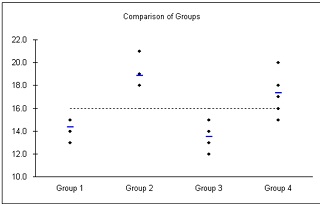
Q3. The City of Maumee comprises four districts. The Chief of Police wants to determine whether there is a difference in the mean number of crimes committed among the four districts. He recorded the number of crimes reported in each district for a sample of six days. (a) At the .05 significance level, can the chief of police conclude there is a difference in the mean number of crimes? (b) What locations differ? (Please identify all pairs!) (c) What multiple comparison test do you use to determine this?
Number of Crimes
Rec Center Key Street Monclova Whitehouse
13 21 12 16
15 18 14 17
14 18 15 18
15 19 13 15
14 18 12 20
15 19 15 18
One factor ANOVA
Mean n Std. Dev
16 14.3 6 0.82 Group 1
16 18.8 6 1.17 Group 2
16 13.5 6 1.38 Group 3
16 17.3 6 1.75 Group 4
16.0 24 2.54 Total
ANOVA table
Source SS df MS F p-value
Treatment 113.00 3 37.667 21.52 1.79E-06
Error 35.00 20 1.750
Total 148.00 23
Post hoc analysis
Tukey simultaneous comparison t-values (d.f. = 20)
Group 3 Group 1 Group 4 Group 2
13.5 14.3 17.3 18.8
Group 3 13.5
Group 1 14.3 1.09
Group 4 17.3 5.02 3.93
Group 2 18.8 6.98 5.89 1.96
critical values for experimentwise error rate:
0.05 2.80
0.01 3.55
p-values for pairwise t-tests
Group 3 Group 1 Group 4 Group 2
13.5 14.3 17.3 18.8
Group 3 13.5
Group 1 14.3 .2882
Group 4 17.3 .0001 .0008
Group 2 18.8 8.91E-07 9.19E-06 .0636
Nonparametric Statistics
Q4. The director of advertising for the Carolina Sun Times, the largest newspaper in the Carolinas, is studying the relationship between the type of community in which a subscriber resides and the portion of the newspaper he or she reads first. For a sample of readers, she collected the following sample information. At the .05 significance level, can we conclude there is a relationship between the type of community where the person resides and the portion of the paper read first? Why?
News Sports Comics
City 170 124 90
Suburb 120 112 100
Rural 130 90 88
Chi-square Contingency Table Test for Independence
Col 1 Col 2 Col 3 Total
Row 1 Observed 170 124 90 384
Expected 157.50 122.25 104.25 384.00
O - E 12.50 1.75 -14.25 0.00
(O - E)² / E 0.99 0.03 1.95 2.96
% of chisq 13.5% 0.3% 26.5% 40.4%
Row 2 Observed 120 112 100 332
Expected 136.17 105.70 90.13 332.00
O - E -16.17 6.30 9.87 0.00
(O - E)² / E 1.92 0.38 1.08 3.38
% of chisq 26.2% 5.1% 14.7% 46.0%
Row 3 Observed 130 90 88 308
Expected 126.33 98.05 83.62 308.00
O - E 3.67 -8.05 4.38 0.00
(O - E)² / E 0.11 0.66 0.23 1.00
% of chisq 1.5% 9.0% 3.1% 13.6%
Total Observed 420 326 278 1024
Expected 420.00 326.00 278.00 1024.00
O - E 0.00 0.00 0.00 0.00
(O - E)² / E 3.02 1.06 3.26 7.34
% of chisq 41.1% 14.5% 44.4% 100.0%
7.34 chi-square
4 df
.1190 p-value
Correlation & Regression
Q5. Mr. James McWhinney, president of Daniel-James Financial Services, believes there is a relationship between the number of client contacts and the dollar amount of sales. To document this assertion, Mr. McWhinney gathered the following sample information. The X column indicates the number of client contacts last month, and the Y column shows the value of sales ($ thousands) last month for each client sampled.
Number of Contacts (X) Sales ($, in thousands) (Y)
14 24
12 14
20 28
16 30
46 80
23 30
48 90
50 85
55 120
50 110
a. Determine the regression equation.
b. Determine the estimated sales if 30 contacts are made.
c. Determine the r square (coefficient of determination)
d. Is there a significant relationship between the number of contacts and sales? Explain your reasoning.
Regression Analysis
r² 0.951 n 10
r 0.975 k 1
Std. Error 9.310 Dep. Var. Y
ANOVA table
Source SS df MS F p-value
Regression 13,555.4248 1 13,555.4248 156.38 1.56E-06
Residual 693.4752 8 86.6844
Total 14,248.9000 9
Regression output confidence interval
variables coefficients std. error t (df=8) p-value 95% lower 95% upper
Intercept -12.2010 6.5596 -1.860 .0999 -27.3275 2.9254
X1 2.1946 0.1755 12.505 1.56E-06 1.7899 2.5993