Case: Major League Baseball Salaries: “Why They Make What They Make”
Background:
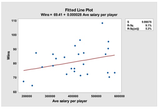
Using the 1986 payrolls and season records, one can easily show the productivity of the players. For example, Table shows a small dataset of all the teams that year. One of the variables is the games won and the other is the average salary of the team. I ran a quick simple linear regression with wins as the dependent variable and average salary as the independent variable. Consider the regression model with these two variables in Figure. One can easily look at the fitted value and the residuals in the table to see who did well and who did not, with the money they paid. If we were to ponder for a moment if player salaries is a good indicator of games won, then it is obvious that this data does not support that hypothesis. First consider the Fitted Line Plot. The relationship is somewhat linear, but the R-squared is very low, meaning that the average salaries do not explain very much of the variation in the number of wins. Also note the hour-glass shape of the scatterplot around the regression line. Analysts far and wide are trying to figure out what is causing that variation.
In Table, it is very easy to see who did good (in the green) and who did bad (in the yellow) that season just by looking at the residuals. (Note: the residual is the actual value minus the predicted value, so a negative residual means that the fitted, or predicted, is actually greater than the actual. Likewise, a positive residual means that the fitted value is less than the actual.) In the National League, based on the amount of money the NY Mets spent, our model predicts that they would win only 84 games. However they won 108 games which is 24 games more than we would have predicted just based on how much money they spent on salaries. In yellow you will see the NL team that did the worst. Our model predicted that Chicago would win 84.4 games, but in reality they only won 70, thus the residual of -14.8. Just based on this data, it is clear that salaries of players are not good indicators of how many games should be won. However, it is relatively easy to see what is driving salaries simply due to their performance variables. These variables consist of things like “At bats”, “#of Home Runs”, “Years in the League” for the hitters, and things like “# of saves” and “ERA” for the pitchers.

For Case we are going to use the 1986 Salary dataset to create a predictive model to predict salaries. This dataset contains 171 pitcher players. (Note: I have trimmed the data set a bit just to get rid of some unusual observations.) Find the excel file and minitab files (Pitchers for Case ) in Canvas.
Case Deliverables:
I. Please submit an Executive Summary of the findings from your data analysis. Also, in the executive summary, provide the general manager any advice that you can based on the data that you analyzed, such as your model and the significant variables. Again, don’t base your advice on your feelings, but purely on the suggestions and conclusions drawn from the data. This section should be very concise and to the point.
II. Create a predictive model using the 5-step methodology used in class and in the text. Step through the process and cut and paste your results from minitab in your report. Throughout your methodology, explain your thought-process and why you make the decisions you make. Give me a narrative of why you are doing what you are doing. I am more interested in your process for model building than the final model that you arrive at.
Although we are interested in using the model for the prediction of baseball salaries, we also want to be able to interpret the contribution of each independent variable in the model. Make sure you provide an interpretation of each coefficient that is in your final model. If you find any weaknesses in your final model after you do your residual analysis in Step 4, be sure to discuss these and perhaps suggest ways to make the model stronger.
Create this model with the 17 original variables provided. Do not do Step 5. Step 5 is “Validation” and to do this you would have to go out and collect more data. There is not a single correct answer/model for this assignment, so I do not expect any two teams to arrive at the same model. If you happen to arrive at the same model, then I wouldn’t expect you to take the same path to that specific model.
Advice: If I recall correctly, I don’t think the “Team” variable is significant in this dataset, so don’t worry about creating a dummy variable for each team. However, the “Position” variable could be interesting. Note that I added a dummy variable to indicate whether the player was a reliever or a starter.
I’m not so concerned about the R-squared value of your final model, but I do think it will be fairly easy for you to get an R-squared value in the 70% to 80% range.
III. Discuss any variable you might like to add to the above model that is not included in the dataset.
IV. If you were the analyst for a team and your general manager wanted to bring in a new reliever (from this dataset), based on your model, who is the best value and who is the worst value. (Hint: you will need to store the Fits and Residuals for your final model.)
Use any of the descriptive statistics tools that you wish from the first portion of the class, such as dot plots, interval plots, histograms, scatter plots, etc., to make your case. Provide accurate interpretations of your findings and try to explain them in simple terms.