Determine the sample correlation coefficient

Question

Assignment:

1. Correlation and Simple Regression the Old-Fashioned Way

This question asks you to compute the sample correlation coefficient (r_xy) and estimate the regression coefficients with ordinary least squares (OLS) "by hand" for the model (Y_i = β₁ + β₂x_i + u_i) using the data below, but without using R (except to get critical values or p-values, and to check your work).

Compute and report the sample correlation coefficient (r_xy).

B. Can you reject the null hypothesis that the true population correlation coefficient is zero at the 5-percent level of significance? Can you reject the null at the 1-percent level of significance? Show your work and explain.

C. Show all of your work in computing the OLS estimates b₁ and b₂.

D. Show all of your work in computing the coefficient of determination (R²) and interpret its meaning.

E. At the 5-percent level of significance, can you reject the null hypothesis that β₂= 0? Can you reject the null hypothesis at the 1-percent level of significance? Show your work and explain.

F. What is the 99-percent confidence interval for β₂? Can you reject the null hypothesis that β₂ = 2 at the 1-percent level of significance? Show your work and explain.

Simple Regression and the Convergence Hypothesis

Many theories of economic growth predict that poorer economies should experience faster rates of economic growth than richer economies. That is, poor economies should converge in per capita income levels to previously richer economies. Convergence is based on three main channels: (1) because of diminishing marginal product of capital, capital should flow from economies with more capital (and a lower marginal return) to countries with lower levels of capital since the marginal impact of an additional unit of capital should be higher in poorer economies, (2) labor should flow from low wage countries to high wage countries helping to equalize wages and reduce differences in per capita incomes, and (3) technology should flow from rich to poor over time, which also allows for convergence.

This question asks you to test the convergence hypothesis using data from 48 U.S. states (each U.S. state is considered as a separate "economy"). I downloaded the data directly from the U.S. Bureau of Economic Analysis website (www.bea.gov), and you can find it as an attachment to this problem set (SAINC4_1929_2018_ALL_AREAS.csv). Note that the data set is "as is". That is, this is the csv file that was downloaded directly from the BEA website.

You need to format the data before you import it into R.

Note that the only data you need for this problem are per capita personal income in 1929 and 2018 for each of the 48 states that were in existence in both 1929 and 2018 (exclude the United States as a whole, Alaska, Hawaii, Washington, D.C., and the regions of the U.S. such as New England, Mideast, etc., since these are not U.S. states. Alaska and Hawaii are deleted since they were not U.S. states in 1929). Here's another hint: Column E in the spreadsheet reports the "LineCode" as a number. For each state, you want line code "30", which is "Per capita personal income (dollars)." So, select the entire spreadsheet and sort by Column E. This will organize this variable for all the states and
territories and you can delete any row from the spreadsheet that is not denoted as line "30".

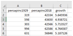
A. Attach your "cleaned" .csv or .xlsx dataset to your submission in Canvas showing the values of personal per capita income for each of the 48 states in both 1929 and 2018. Below is a screen shot of my *.csv file with personal income per capita in 1929, personal per capita income in 2018, and the average annual growth rate (in percent) between 1929 and 2018  3 (see Part B below), with each of the 48 states in alphabetical order. Row 2, for example, is Alabama:

Create a well-labeled and well-formatted, two-variable scatter diagram in R for all 48 U.S. states with the plot() command in R. I have provided an example of a script for a scatter diagram in R. The level of per capita personal income in 1929 (in dollars) by state should be on the horizontal axis while the average annual growth rate of per capita income by state from 1929 to 2018 on the vertical axis. You can compute the average annual growth rate from 1929 to 2018 for each state using the following formula. It is easier to compute growth rates in Excel before you import the data set into R, but you can do it in R too:

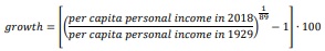
The formula above computes the average annual growth rate in percent. For example, you should get ≈ 5.645936 percent for Alabama as shown in Part A above. That is, nominal per capita income increased at approximately 5.645936 percent per year from 1929 to 2018. Your data set in R should consist of 48 cross-sectional observations for the variable growth for each state and the variable per capita personal income in 1929 for each state.

Is your scatter diagram consistent with the convergence hypothesis? Briefly explain.

C. Estimate and report, using stargazer, the following OLS regression model:

growth = b₁+b₂ per capita personal income in 1929

With stargazer, report the coefficients to the fifth decimal point, with the embedded command digits=5.

D. Formally test the convergence hypothesis, using a t-test at the 1-percent level of significance. What are the null and alternative hypotheses? Can you reject the null? Are your results consistent with the convergence hypothesis at the 1-percent level of significance? Explain.

3. Wages and Physical Attractiveness: Using R to Estimate an OLS Multiple Regression

A. Use the attached data set looks.csv to estimate and report a multiple regression model with R using ordinary least squares and the package
stargazer to format the regression results. In the table created with stargazer, set the digits=5 to show the results to the fifth decimal point.
The dependent variable is the natural logarithm of wages (lwage). The explanatory variables are all listed in the csv file.

B. Are the signs of the estimated coefficients consistent with economic theory and your intuition? Explain. Which estimated coefficients are statistically different from zero at the 1-percent level of significance? Explain.

C. Interpret the precise meaning of the estimated coefficient on years of schooling (educ).

D. Using the results from Part A, at how many years of experience are lwages (and wages) maximized? Does this answer seem plausible? Show your work and explain.

E. Suppose someone claims that a one-unit increase in looks (physical attractiveness) on a five-point scale is associated with more than a ten-
percent increase in wages. What are the null and alternative hypotheses?

Can you reject this null hypothesis at the 5-percent level of significance?

Can you reject this null hypothesis at the 1-percent level of significance?

Show your work and explain.

4. Weight Gain in College: Interpreting OLS Multiple Regression Output

The table labeled Table below is from the published paper, "The Freshman 15:

A Critical Time for Obesity Intervention or Media Myth?," by Jay L. Zagorsky and Patricia K. Smith (Social Science Quarterly 92(5), December 2011, pp. 1389- 1407). It uses a nationally representative random sample, from the National Longitudinal Survey of Youth (NLSY97), to estimate the weight change (in pounds) during college.

A. Consider an unmarried, white, male, part-time college student who is 23 years of age and who has been in college for five years at a four-year (BA- granting) college. He worked 50 weeks last year for pay and his family income is $40,000 (or 40 since the footnote to the table says that income is measured in $1,000 increments) so he is not living in poverty. He attends a private school in the northern United States, and he lived in the dorms his freshman year although he does not consider himself to be a heavy drinker. Based on regression (4) above, what is his predicted weight gain since starting college? Show your work.

B. Suppose that an expert in nutrition claims that, all else equal, each year of college leads to a five-pound weight gain. Using the results from
regression (4) above, what is the value of the test statistic associated with this null hypothesis? Can you reject this null hypothesis at the five- percent level of significance? Can you reject this null hypothesis at the one-percent level of significance? Note that since the sample is so large, the distribution is approximately standard normal with a value of 1.96 for the two-sided 5-percent critical value and 2.58 for the two-sided 1-percent critical value. Briefly explain.

C. Which of the variables in Table above are dummy variables? Briefly explain.

Attachment:- Cleaned Dataset.rar