Problem 1: Decision Making using Decision Tables
Fred and George are recent graduates who met while they were studying degrees in IT and business respectively. They are considering setting up a small tutoring agency to provide assistance to school students in subjects such as mathematics and accounting. Their biggest expense in setting up their agency is the cost of renting office space that they can use to deliver their tutoring services.
In their search for a suitable office, they have come across two offices which would be suitable. One is fairly expensive, but is located close to many schools, so it is likely they would have many students seeking their services. The other office is less expensive, but not so conveniently located.
They have done some modelling, and have estimated that in a favourable market, renting the more expensive office would allow them to generate a net profit of $10,000 over two years; but if the market was unfavourable, they could lose $8,000. On the other hand, renting the less expensive office would generate a return of $7,000 over the two years if the market was favourable, but they would lose $2,000 in an unfavourable market. Since the overall economic outlook is positive, they have estimated that there is a 60% chance that the market will be favourable.
They need to decide among the following three alternatives: Alternative A: Rent the more expensive office Alternative B: Rent the less expensive office
Alternative C: Do nothing; i.e., don't set up the business.
Answer the following questions:
a) Which alternative would be chosen under a maximax decision procedure? Explain how you arrived at this answer.
b) Which alternative would be chosen under a maximin decision procedure? Explain how you arrived at this answer.
c) Given that George tends to be risk averse, what would his decision be? Relate your answer to the answers you have given to the first two questions.
d) What would their decision be if they were to choose the alternative with the greatest expected value? Show all calculations, and justify your answer.
Fred and George would like to see how their decision would be affected if the probability of a favourable market was some other value than 60%.
e) Construct a plot showing how the expected value of the returns for Strategy 1 and Strategy 2 vary with the value of P (for 0 ≤ P ≤ 1), where P is the probability of a favourable market.
f) Find the range of values for P for which the following decisions would be made. You can estimate values from the plot in (e).
i. Strategy 1
ii. Strategy 2
iii. Strategy 3
Fred and George know a person who claims to be able to predict with absolute certainty whether or not the market will be favourable, but he will only provide this information for a cost.
g) Assuming that this person's prediction is always correct, what is the maximum amount that Fred and George should be willing to pay for this information? You must explain your reasoning clearly.
Problem 2: Optimizing an advertising program
The Big Bet is a new online sports betting agency. Jane Simmons is the marketing manager, and has a $30,000 limit available to spend on advertising for the next week, with the objective of attracting as many new customers has possible. She would like to spend this advertising budget over four types of adds: television ads, radio ads, billboard ads and newspaper ads.
Her research has provided the following information: a TV ad costs $1,250 and reaches an estimated audience of 30,000 viewers; a radio ad costs $550 and reaches an estimated audience of 22,000 viewers; a billboard ad cost $500 and reach an estimated audience of 24,000 viewers, and a newspaper ad costs $150 and reaches an estimated audience of 8,000 viewers.
There are several constraints that she wishes to impose on how she distributes the $30,000.
- She does not want to be overexposed in any one form of advertising, so she must place no more than 20 ads of each type.
- The amount spent on billboards and newspapers together must not exceed the amount spent on TV ads
- Due to contractual arrangements, she must place at least 10 ads per week on TV or radio or some combination of the two.
Jane's Question is to determine how many ads of each type should be placed in order to maximise the total number of people reached.
Your task is to set this Question up as a linear programming Question, and solve it in Excel using the Solver linear programming add-on for Excel.
Use your model to answer the following:
- How many ads of each type should be placed in order to maximise the total number of people reached?
- What is the number of people reached by placing these ads?
- What is the total cost of placing these ads?
Gina is the inventory manager for an electronics store that sells a variety of electronic devices. For the last twelve months, the store has been stocking a Problem 3: Using Simulation to Estimate Cost of Inventory Policy
product called the SoundStation, which is a premium quality wireless speaker than can be connected to remotely from mobile phones, iPads, etc. The SoundStation has proved to be very popular with customers and they have been selling well, despite their relatively expensive price.
A Question for Gina is that several similar products are soon going to go to market, and this will mean that sales of the SoundStation will decrease; however it is not known when these new products will become available. Gina does not want to miss out on sales of the SoundStation, so she would like to maintain a sufficient stock level. However she does not want to keep too much stock, because once the new products are released she may not be able to sell her remaining inventory of the SoundStation.
Gina would like to develop an inventory policy for the SoundStation.
The Question contains a number of probabilistic variables, and thus Gina would like to set up a simulation model to help her explore various inventory policies.
Daily demand for the SoundStation is subject to variability, and is thus a probabilistic variable. Table I shows the daily demand for the SoundStation over the past 200 days. From this table Gina can estimate, for example, that the probability of that there will be a demand for one unit of the SoundStation on any particular day is 0.3 (i.e. 60/200).
Table I: Demand and frequency for SoundStation
|
Demand
|
0
|
1
|
2
|
3
|
4
|
|
Frequency (days)
|
30
|
60
|
75
|
25
|
10
|
When Gina places an order to replenish her inventory of the SoundStation, it can take anywhere between 1 and 3 days for the stock to be delivered to the store; i.e., there is a 1 to 3 day lead time. Thus, lead time can also be considered a probabilistic variable. If the lead time for the order is 1 day, the order will not arrive the next morning, but at the beginning of the following working day. For example, assuming an order is placed on a Monday, if the lead time is 1 day the stock will arrive on the Wednesday; if the lead time is 2 days then the stock will arrive on the Thursday, and so on.
Table II shows the lead time for the last 50 orders that Gina has placed. From this table Gina can estimate, for example, that the probability of receiving new stock exactly two days after an order has been placed is 0.50.
Table II: Lead time and frequency for SoundStation orders
|
Lead Time
|
1
|
2
|
3
|
|
Frequency (orders)
|
10
|
25
|
15
|
Gina is considering the following inventory policy. Whenever the day's ending inventory reaches the re-order point of 5 units and there are no outstanding orders which have not yet arrived, Gina requests an additional 10 units from her supplier (i.e., the re-order quantity is 10). A 6-day snippet of the simulation is shown in Table III.
Table III: Simulation of SoundStation inventory for 6 days
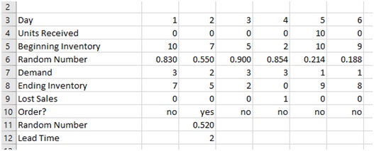
Here is an explanation of the simulation in the above table. It is assumed that the beginning inventory is 10 units (i.e., the re-order quantity). Since the demand on day 1 is 3 units, the ending inventory on day 1 is 7. This is above the re-order point of 5 units, so no order is placed on day 1. Since the demand on day 2 is 2 units, the ending inventory will be 5 units, and thus an order for 10 units will be placed. The lead time for the order is 2, which means that the 10 ordered units will not be received until day 5. There is a lost sale of 1 unit on day 4 because the demand on day 4 is 3 units, but the beginning inventory is only 2 units. Note that although the ending inventory on days 3 and 4 is below the re-order level, no orders are placed on these days because there is an outstanding order from day 2 which has not yet arrived.
There are various costs associated with the inventory policy.
- The cost of placing an order is $50 and covers costs of delivery, etc.
(This is a fixed cost and does not depend on the number of items in the order).
- The cost of holding a SoundStation in stock is $2 per unit per day (This covers costs of insurance, storage, etc.)
- The cost of each lost sale is $100
(This is not a real cost; it is the profit that is missed out on because the customer will buy the product elsewhere).
Gina can easily calculate these costs from the spreadsheet above. For example, it can be seen that over the 6 days 2 orders have been placed (2 x $50 = $100); 21 units have been held in stock (21 x $2 = $42); and there have been 4 lost sales (4 x $100 = $400). Thus the effective cost over the 6 days is thus $542.
(a) Gina would like to know the yearly cost of this inventory policy.
Implement the policy using a spreadsheet, run a 200-day simulation (the electronics store is open for 200 days a year), and estimate the yearly inventory cost. Note that you will probably observe considerable variability between different simulation trials. Run several trials (say, 20), and calculate the average yearly inventory cost and the standard deviation of the yearly inventory cost. (For information on how to find the average and standard deviation, refer back to Activity 3 from the Week 2 lab).
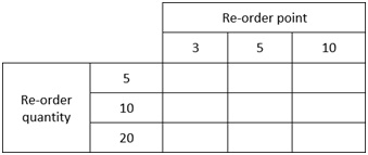
(b) Gina would like to experiment with some other values for re-order point and re-order quantity.
Complete the table below with the estimated cost corresponding to each combination of values for re-order point and re-order quantity. Once again, each of these should be the average over a sufficient number of trials. Include both the average and the standard deviation in the table.
(c) Based on your results what would you recommend to Gina? Should she change her inventory policy?
Attachment:- Decision Support Systems.rar