--%>

Sample Questions in Graphical Solution Procedure

Solved problems in Graphical Solution Procedure, sample assignments and homework

Questions: Minimize Z = 10x1 + 4x2

Subject to

3x1 + 2x2 ≥ 60

            7x1 + 2x2 ≥ 84

            3x1 +6x2 ≥ 72

x1 ≥ 0 , x2 ≥ 0


Answer

The first constraint 3x1 + 2x2 ≥ 60, can be written in form of equation

3x1 + 2x2 = 60

Place x1 =0, then x2 = 30

Place x2 =0, then x1 = 20

Then the coordinates are (0, 30) and (20, 0)


The second constraint 7x1 + 2x2 ≥ 84, can be written in form of equation

7x1 + 2x2 = 84

Place x1 =0, then x2 = 42

Place x2 =0, then x1 = 12

The coordinates then are (0, 42) and (12, 0)


The third constraint 3x1 +6x2 ≥ 72, can be written in form of equation

3x1 +6x2 = 72

Place x1 =0, then x2 = 12

Place x2 =0, then x1 = 24

Thus, coordinates are (0, 12) and (24, 0)


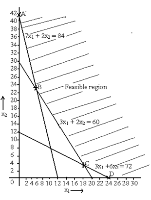
The graphical presentation is
 

 1485_Graphical Solution Procedure Sample Assignment.png 


The corner positions of feasible region are A, B, C and D. Thus the coordinates for the corner points are

A (0, 42)

B (6, 21) (Solve the two equations 7x1 + 2x2 = 84 and 3x1 + 2x2 = 60 to obtain the coordinates)

C (18, 3) Solve the two equations 3x1 +6x2 = 72 and 3x1 + 2x2 = 60 to obtain the coordinates)

D (24, 0)


We are given that Min Z = 10x1 + 4x2

At A (0, 42)

Z = 10(0) + 4(42) = 168


At B (6, 21)

Z = 10(6) + 4(21) = 144


At C (18, 3)

Z = 10(18) + 4(3) = 192


At D (24, 0)

Z = 10(24) + 4(0) = 240


The minimum value is calculated at the point B. Consequently Min Z = 144 and x1 = 6, x2 = 21

   Related Questions in Basic Statistics

  • Q : Model Checking Approach Model Checking

    Model Checking Approach: • Specify program model and exhaustively evaluate that model against a speci?cation        –Check that properties hold   

  • Q : Explain Queuing theory Queuing theory :

    Queuing theory: • Queuing theory deals with the analysis of lines where customers wait to receive a service:

    Q : Problem on queuing diagram Draw a 

    Draw a queuing diagram for the systems below and describe them using Kendall’s notation: A) Single CPU system <

  • Q : State Littles Law Little’s Law : • L =

    Little’s Law: • L = λR = XR • Lq = λW = XW • Steady state system • Little’s Law holds as long as customers are not destroyed or&nbs

  • Q : MANOVA and Reflection Activity

    Activity 10:   MANOVA and Reflection   4Comparison of Multiple Outcome Variables This activity introduces you to a very common technique - MANOVA. MANOVA is simply an extension of an ANOV

  • Q : Probability how can i calculate

    how can i calculate cumulative probabilities of survival

  • Q : Assumptions in Queuing system

    Assumptions in Queuing system: • Flow balance implies that the number of arrivals in an observation period is equal to the

  • Q : FIN512 Entrepreneurial Finance Chapter

      Chapter 6: Discussion Question: #4 p. 223  It is usually easier to forecast sales for a seasoned firm contrast to an early-stage venture because an early-stage venture has limited access to bank credit lines, sho

  • Q : Cumulative Frequency and Relative

    Explain differences between Cumulative Frequency and Relative Frequency?

  • Q : Explain Service times Service times: A)

    Service times:A) In most cases, servicing a request takes a “short” time, but in a few occasions requests take much longer.B) The probability of completing a service request by time t, is independent of how much tim