Assignment:
Case Problem 1
Data File needed for this Case Problem: Popcorn.xlsx Ride}, Popcorn Ricky Nolan established Ricky's Popcorn in Havahorne, Nevada, in 2000. He ships flavored popcorn in standard flavors such as plain and kettle corn and gourmet flavors such as grape and orange. Customers place their orders via the company website and then receive their popcorn in one to three days, depending on the shipping option they choose. Ricky wants to create a professional-looking invoice he can use for each customer tran.ction. Ricky used Excel to create the invoice layout and wants you to add formulas to calculate the price per item, .les tax, shipping, and invoice total based on existing tables thr pricing and shipping. Complete the following:
1. Open the Popcorn workbook located in the Exce18 > Casel folder included with your Data Fil., and then save the workbook as Ridcys Popcorn in the location specified by your instructor.
2. In the Documentation WorkSheet, enter your name and the date.
3. In the Pricing and Shipping worksheet, auign the defined name Shipping.. to the data in the range D3:E7, which can be used for an approximate match lookup. (Hint: The lookup table includes only the valu., not the d.criptive labels.)
4. In the Customer Invoice worksheet, in the Item column (range B16:826), u. data validation to create a list of the items in the Product Pricing table in the Pricing and Shipping worksheet. (Hint: Select the entire range before .tting the validation rule.)
5. In the Flavor colurnn (range E16:E26), u. data validation to create an input meuage indicating that the popcorn flavor should be entered. The flavors are located below the invoice.
6. In the Price cell (cell G16), u. a VLOOKUP function to r.rieve the price of the ordered item listed in the Product Pricing table in the Pricing and Shipping worksheet. (Hint: U. the defined name ProductPrice that was assigned to the Product Pricing table.) When no item is selected, this cell will display an error message.
7. Modify the formula in the cell G16 by combining the IFERROR function with the VLOOKUP function to display either the price or a blank cell if an error value occurs. Copy the formula down the range G16:G26.
8. In the Total column (range H16:H26), enter a formula to calculate the total charge for that row (Qty x Price). Use the IFERROR function to display either the total charge or a blank cell if an error value occurs.
9. In the Subtotal cell (cell H27), add a formula to sum the Total column. U. the IFERROR function to display either the subtotal or a blank cell if an error value occurs.
10. In the Sal.Tax cell (cell H28), enter a thrmula with an IF function so if the customer's state (cell C12) is NV, then calculate 6.85 percent of the subtotal (cell H2, otherwise, u. 0 for the .1. tax. (Hint: The defined name State is auigned to cell C12, and the defined name Sub_Total is assigned to cell H27. Note that the defined name "Sub_Total" is intentionally not spelled as "Subtotal," which is the name of an Excel function.)
11. In the Shipping cell (cell H29), enter a formula that n.ts theVLOOKUP function in an IF function to look up the shipping cost from the Shipping Cost table in the Pricing and Shipping worksheet based on the subto.I in cell H27. If the subtotal is 0, the shipping ct should diplay O. (Hint U. the defined name you created for the Shipping Cost table data.)
12. In the To.I Due cell (cell H30), calculate the invoice total by entering a formula that adds the valu. in the Subtotal, Sal. Tax, and Shipping cells.
13. Test the worksheet by using the following order data:
• Sold to: Lauri Bradford
• Street: 3226 South Street
• City, State Zip: Hawthorne, NV 89415
• Date: 12/1/2017
• Item 1: Gourmet (2) 1g
• Flavor: Nacho Cheese
• Quantity 2
• Item 2: Plain Tin lg
• Quantity: 1
14. Save the workbook, and then close it.
Case Problem 2
Data File needed for this Case Problem: Athey.xlsx
Miley Department Sto AtheyCfeparrrn in Fort Dodge, Iowa, has alwaysacceptedeturns product purchased in oe4t:ttoe for the V returns. A routing slip will allow him to monitor who handled the return at each step. He will also be able to collect the returns data in a worksheet for count of returns in each category. Mitchell has started developing the routing slip, and he wants you to finish creating it. Complete the following:
1. 0pen the Athey workbook located in the Excel8 > Case4 folder included with your Data Files, and then save the workbook as Athey Routing Slip in the location specified by your instructor.
2. In the Documentation worksheet, enter your name and the date.
3. Create a defined name for the table on the Return Data worksheet to help you when you create formulas with VLOOKUP functions. (Hint: U. a name other than ReturnTbl because this name is already used as the defined name for the table on the Return Data worksheet.)
4. In the Return Routing worksheet, do the following:
a. In cell B9, use a date function to display the current date.
b. In cell B11, use an input message to inform the user to enter a product description in this cell.
c. In cell B14, use a list validation for the Department located on the Return Data worksheet.
d. In cell B16, use a list validation for the Resolution located on the Return Table worksheet (the range B1:E1).
e. In cell B20, use an input message to inform the person entering the information to enter their name, initials, or Employee ID in this area.
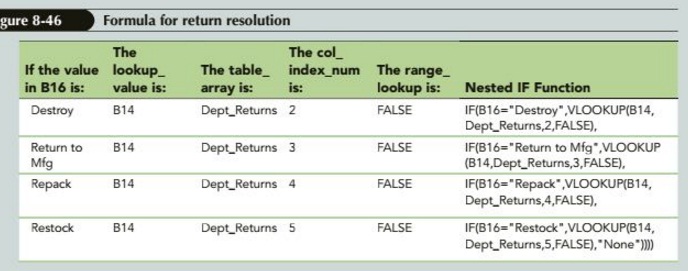
5. In cell B18, create a formula using nested IF functions and VLOOKUP functions to determine what to do with the returns. Use the lookup table in the Return Data worksheet. Refer to Figure .6 for some hints on how to create the formula.
6. Test your routing slip by entering the following information:
• Product Name: Deluxe Vacuum
• Department: Electronics
• Resolution: Return to Mfg
• Customer Assistant: 01265
7. Protect all cells in the Return Routing worksheet except those in which you enter data.
8. In the Return Analysis worksheet, complete the following analysis of the Return Data worksheet using COUNTIF:
a. Compute the total Retums by Department.
b. Compute the total Returns by Resolution.
9. Save the workbook, and then close it.
Attachment:- Athey Department Store.xls