1) The t and F Distributions
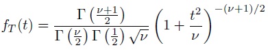
The T random variable with v degrees of freedom has the distribution
Show that the random variable F = T2 has the F distribution with 1 and v degrees of freedom.
2) An Unbiased Estimate of σ
The chi distribution models the square root of a chi-square random variable:
Y= √x X~ x2 v
(a) Find the pdf of the chi distribution.
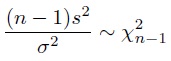
(b) We know that the sample variance from a normal distribution follows a chi-square distribution
Find the expected value of the sample standard deviation, s, and suggest an adjustment that would make it unbiased. You may find the following formulas useful:

3) A Catch-and-Release Estimate
A park has N raccoons of which 10 were previously captured and tagged. Suppose that 20 raccoons are captured. Find the probability that n = 5 of these are found to be tagged. Denote this probability by p(N).
(a) Find the value of N that maximizes p(N); this is called a maximum likelihood estimate. Hint: compare the ratio p(N)/p(N -1) to unity.
(b) Plot the maximum likelihood estimate of N against varying values of n, from 1 to 10.
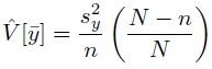
4) Finite Population Correction Factor
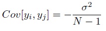
For a finite population of size N with mean µ and variance σ2, it can be shown that the covariance of any two observations in a sample is
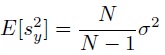
and that the sample variance is slightly biased
This means that the variance of the sample mean, when drawn from a finite population, includes a covariance term. This gives rise to the finite population correction factor. Use these relationships to show that the variance of the sample mean is
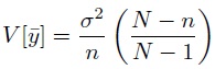
and that this is estimated by
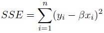
5) Zero-Intercept Regression
Some phenomena follow a linear model which has an inherent zero response for a zero predictor, so the candidate regression model is
y=βx+ε
(a) Find the ordinary least squares estimator for β by minimizing the sum of squared errors
(b) It seems reasonable that the variance around the regression line would increase as the predictor increases (think of the line swinging around the fixed "pivot" at the origin). If the error was normally distributed, this could give rise to the conditional distribution
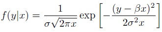
Assuming this distribution, find the maximum likelihood estimator for β .
Explain why this is called a ratio estimator.
(c) for the following data, estimate β using both your OLS and MLE estimators.
x 0.5 1.5 3.2 4.2 5.1 6.5
y 1.3 3.4 6.7 8.0 10.0 13.2
6) A Truncated Distribution
Students in several statistics classes were asked to complete a questionnaire. One of the quantities asked was the number of siblings a student had. This is a summary of the responses:
siblings frequency
0 4
1 22
2 22
3 11
4 8
5 3
6 3
12 1
20 1
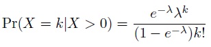
6.1) Problem. Use the sibling data to estimate a distribution for the number of children in a family. Obviously, the number of children is one more than the number of siblings. However, there is a selection bias in this measurement; families with no children cannot be reported this way! Therefore the data follows a zero-truncated Poisson distribution (ZTPD)
(a) Find the MLE for the parameter λ of the ZTPD.
(b) What are the mean and variance of the ZTPD? Rather than directly calculating the moments, you might find it simpler to use the probability generating function
Gk(z) = E[zk]
and then take advantage of the properties of the pgf:
E[K] = G'k(z = 1) V ar[K] = G"k(z = 1) + G'k(z = 1)- [G'k(z=1)]2
(c) Estimate the mean for the number of children and determine whether the data fits a ZTPD with that mean.
7) Estimating with Confidence The times to failure (in hours) for a sample of n = 30 backup generators are
7494.7 8801.7 9990.7 11277.7 10173.3 7746.8
9003.6 8242.9 4532.2 12541.8 6766.9 9898.9
8922.0 13429.8 17623.5 9135.6 6029.8 9038.7
20972.0 7605.1 5396.6 7528.2 10330.6 6475.4
12390.9 9857.0 7067.6 9704.2 5055.8 9942.4
(a) Find the mean time to failure and a 95% confidence interval (use a t distribution).
(b) Find a 95% confidence interval for the standard deviation (start with a chi-square interval for the variance).