Solve the following problem:
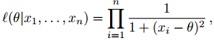
For the Cauchy likelihood of Example 1, based on a simulated sample of size n = 100, show that the pseudo-posterior distribution πm(θ|x) ∝ l(θ|x)m is defined for any integer m > 0. Using integrate to properly normalize πm, show graphically how πm concentrates as m increases.
Example 1:
When considering maximizing the likelihood of a Cauchy C(θ, 1) sample,
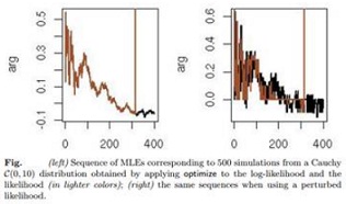
the sequence of maxima (i.e., of the MLEs) is converging to θ ∗ = 0 when n goes to ∞. This is reflected by Figure (left), which corresponds to the code
> xm=rcauchy(500)
> f=function(y) {-sum(log(1+(x-y)ˆ2))}
> for (i in 1:500){
+ x=xm[1:i]
+ mi=optimise(f,interval=c(-10,10),max=T)$max}
where the log-likelihood is maximized sequentially as the sample increases. However, when looking directly at the likelihood, using optimise eventually produces a diverging sequence since the likelihood gets too small around n = 300 observations, even though the sequences of MLEs are the same up to this point for both functions. When we replace the smooth likelihood with a perturbed version, as in
> f=function(y){-sin(y*100)^2-sum(log(1+(x-y)^2))}
the optimise function gets much less stable, as demonstrated in Figure (right), since the two sequences of MLEs (corresponding to the log-likelihood and the likelihood) are no longer identical.