Problem 1
Use the following four data sets for problem 1 (from Anscombe (1973), American Statistician). Be aware that this is a very interesting series of data sets with some special properties. I do not have data files for these data, so you’ll need to enter it by hand. If you want to challenge yourself, try to copy and paste this data into an excel sheet or text file and then bring it in through SPSS.
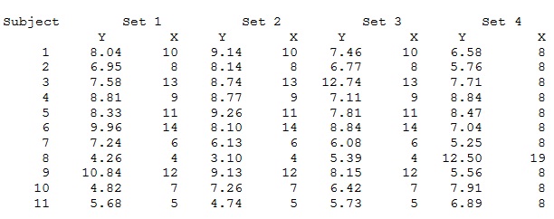
(a) For each of the four data sets separately: Calculate the Pearson r and the regression equation, = b0 + b1X; Calculate R2 and associated test of significance. Test b1 for significance. Briefly write what you would conclude about the comparison of these datasets from these analyses.
(b) For data set 1 and data set 3, compute the outlier diagnostics. Are there are any outliers? If so, please explain.
(c) Comment on what lessons have you learned (or should have learned) from this problem. That is, why did I pick these data and ask you to specifically do steps a, &b? When looking at the data analysis as a whole, what lesson should this question teach?
Problem 2
The following are actual data showing the latitude of a sample of major cities in the northern hemisphere and their mean high annual temperature.
latitude(X) mean high temp(Y)
1. Acapulco 17 88
2. Algiers 37 76
3. Berlin 53 55
4. Bogota 5 66
5. Montreal 46 50
6. Oslo 60 50
7. Rome 42 71
8. Saigon* 11 90
* Now known as Ho Chi Minh City.
(a) Compute and write the prediction regression equation(note: do not just refer to spss output—write out the full equations)
(i) In unstandardized form (For every increase in ___, x goes up by ____)
(ii) In standardized form(units)
(b) Calculate the predicted mean temperature (degrees F) for each city.
(c) Test the b1 coefficient; Calculate and test R2
Report results of these tests in a short APA results-style paragraph
(d) Plot Y (vertical axis) vs. X (horizontal axis) showing best fitting straight line
(e) Report standard measures of leverage (X space), studentized deleted residuals (Y space), and SDFFITS (influence) for each city.
(f) Examine your plots. Consider your expectations, the obtained values of r and b1, the plots, and your outlier statistics. Do any of the cities appear to be having a particularly strong influence on the results? If so, which one(s) and why?
(g) Drop the point(s) identified in (f) from the data analysis and using SPSS re-compute r and b1. Test the new b1 coefficient; Calculate and test the new R2.Report the results of these tests in a short APA results-style paragraph, and describehow do the results change?
(h) In general, are you justified in dropping data? When is it appropriate vs. inappropriate? Comment on why this procedure of dropping one or more cities may or may not be appropriate in the present case (Hint: consider the altitudes—not latitudes-- of the cities).
Problem 3
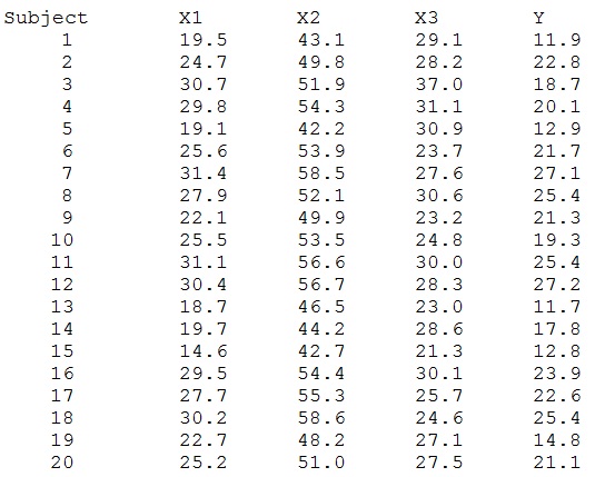
The following data are measures of triceps skinfold thickness (X1), thigh circumference (X2), and midarm circumference (X3). These three variables are used to predict percentage of body fat (Y). You can also find the data on beachboard (titled “bodyfat”).
(a) Compute the regression of Y on X1.
(b) Compute the regression of Y on X2.
(c) Compute the regression of Y on X1, X2
(d) Compute the regression of Y on X1, X2, X3
In each case, report the results in a brief APA results-style paragraph. For each individual predictor remember to report bs, standard error of each b (or confidence intervals), t test; and for each overall model report F test,df, and R2.
(e) Compute the correlation matrix of the predictors (X1 X3)
(f) Compute the tolerance (or VIF) of each predictor for the equation (d) which includes all 3 predictors.
(g) Examine the outlier statistics for the X space, Y space, and influence (including DFBETAS for each predictor). Identify the highly discrepant observations, if any.
(h) Comment on what you have learned about this data set, particularly with regard to the three predictors, and interpret the results.
Problem 4
Data for problem 4 are provided by Tabachnik&Fidell (2007), and represent a subset of variables that were collected as part of a year-long study on the relationship between stressful life events and mental and physical health (for more details on this study see Appendix B1 of Tabachnik&Fidell , 2007 or see Hoffman &Fidell, 1979, where these data were initially published). You can find the five variable data set (N= 465) on beachboard(titled “tbregress”). Here is a brief description of the variables:
subjno: Subject number
timedrs: number of visits to health professionals over the course of the study
phyheal: self reported frequency count of problems with various body systems (circulation, digestion, etc.), general description of health
menheal: frequency count of mental health problems (feeling somewhat apart, can’t get along, etc.)
stress: weighted items reflecting number and importance of change in life situation
Use multiple regression and correlation analyses to understand what the data from these variables tell us about the relationships between mental and physical health. Remember to use data centering to make sense of your data (when you want to make the intercept values meaningful). Clearly state the research questions that you want to test in these data and describe the results from the statistics you used to test your models. Write your work as a results section, organized by the research question you are testing.